In the DDIM post, setting $\sigma_t = 0$ turned the DDPM sampler into a deterministic map from noise to data. A deterministic map that moves a point a little at each step is an ODE. Flow matching starts from that ODE: instead of deriving it from a noising process, it picks the path from noise to data first, and trains a network to output the velocity along it.

Most recent image and video generators (Stable Diffusion 3, FLUX, many video models) are trained this way. It is also the starting point for almost every one-step method in the next post.

1. One notation for both

This post uses the convention of rectified flow, SD3 and MeanFlow: $t = 0$ is data and $t = 1$ is noise, the same direction as DDPM, where larger $t$ means noisier.

\begin{equation} x_t = \alpha_t\, x_0 + \sigma_t\, \epsilon, \qquad x_0 \sim p_{\text{data}},\quad \epsilon \sim \mathcal{N}(0, \mathbf{I}) \end{equation}

• DDPM / DDIM (variance preserving): $\alpha_t = \sqrt{\bar\alpha_t}$, $\sigma_t = \sqrt{1-\bar\alpha_t}$. (The DDIM post wrote $\alpha_t$ for what is $\bar\alpha_t$ here.)
• Flow matching with the linear path (rectified flow): $\alpha_t = 1 - t$, $\sigma_t = t$, so $x_t = (1-t)\,x_0 + t\,\epsilon$.

The second one is a straight line from each data point to each noise sample. That is the whole design.

2. What the network learns

Conditional velocity #

Pick one pair $(x_0, \epsilon)$. Along its path, the velocity is just the time derivative:

\begin{equation} \frac{d x_t}{d t} = \dot\alpha_t\, x_0 + \dot\sigma_t\, \epsilon \;\overset{\text{linear}}{=}\; \epsilon - x_0 \end{equation}

For the linear path it is constant in time: a straight line at constant speed.

Marginal velocity #

At sampling time we don’t know which $(x_0, \epsilon)$ produced a given $x_t$. Many pairs pass through the same point. The velocity field that actually moves the whole distribution $p_t$ is the average of the conditional velocities over all pairs that pass through $x$ at time $t$:

\begin{equation} v(x, t) = \mathbb{E}\left[\, \epsilon - x_0 \;\middle|\; x_t = x \,\right] \end{equation}

This field satisfies the continuity equation $\partial_t p_t + \nabla\cdot(p_t\, v) = 0$, which means: if you start with samples of $p_1 = \mathcal{N}(0, \mathbf{I})$ and integrate $\frac{dx}{dt} = v(x,t)$ from $t=1$ down to $t=0$, you end with samples of $p_0 = p_{\text{data}}$.

The loss: regress on the conditional target #

We can’t compute $v(x,t)$ directly, because it needs the posterior over $(x_0, \epsilon)$. The key fact of flow matching (Lipman et al.) is that we don’t need to. Train on the conditional target:

\begin{equation} \mathcal{L}_{\text{CFM}}(\theta) = \mathbb{E}_{t,\, x_0,\, \epsilon}\left\| v_\theta(x_t, t) - (\epsilon - x_0) \right\|^2 \end{equation}

Why it works. Expand the square. The term $\|v_\theta\|^2$ is the same as in the loss we actually want, $\mathbb{E}\|v_\theta(x_t,t) - v(x_t,t)\|^2$. The cross term is

\begin{equation} \mathbb{E}_{x_t}\Big\langle v_\theta(x_t,t),\; \mathbb{E}[\epsilon - x_0 \mid x_t] \Big\rangle = \mathbb{E}_{x_t}\big\langle v_\theta(x_t,t),\; v(x_t,t) \big\rangle \end{equation}

by the tower property. The remaining terms don’t depend on $\theta$. So the two losses differ by a constant and have the same gradients, and the minimizer is exactly the conditional expectation $v_\theta^\star(x,t) = v(x,t)$.

3. Flow matching is diffusion, reparameterized

For a Gaussian path, the network’s output can be converted between all the usual targets. For the linear path, given a velocity prediction $\hat v$:

\begin{align} \hat x_0 &= x_t - t\,\hat v \\ \hat\epsilon &= x_t + (1-t)\,\hat v \\ \nabla_x \log p_t(x_t) &= -\,\hat\epsilon / t \end{align}

So an $\epsilon$-prediction network, an $x_0$-prediction network, a score network and a velocity network trained on the same path all represent the same field. What actually differs between “diffusion” and “flow matching” papers is:

1. the schedule $(\alpha_t, \sigma_t)$,
2. which quantity the network outputs (this changes the effective loss weighting over $t$),
3. how $t$ is sampled during training.

Kingma & Gao showed that these choices amount to different weightings of the same ELBO-like objective. SiT (Ma et al.) explored the design space with one transformer and found the linear interpolant with velocity prediction a strong default.

DDIM is Euler on this ODE #

Here is the link back to the previous post. A DDIM step from $t$ to $s < t$ with $\sigma = 0$ predicts $\hat x_0$ and $\hat\epsilon$, then re-noises to level $s$:

\begin{equation} x_s = \alpha_s\, \hat x_0 + \sigma_s\, \hat\epsilon \end{equation}

With the linear path, substitute the conversions above:

\begin{equation} x_s = (1-s)(x_t - t\hat v) + s\,(x_t + (1-t)\hat v) = x_t + (s - t)\,\hat v \end{equation}

That is exactly one Euler step of $\frac{dx}{dt} = v$. For other schedules DDIM is still an Euler step, in the rescaled coordinates $x/\alpha$ against $\sigma/\alpha$. DDIM was a flow sampler all along.

4. Straight training paths, curved sampling paths

If every training path is a straight line, why do we still need 20-50 steps?

Because the network does not learn the straight lines. It learns their average, and the average of crossing lines is not straight. The figure below is computed exactly for a 1-D toy dataset with two modes at $\pm 1$ (for a Gaussian mixture the marginal velocity has a closed form).

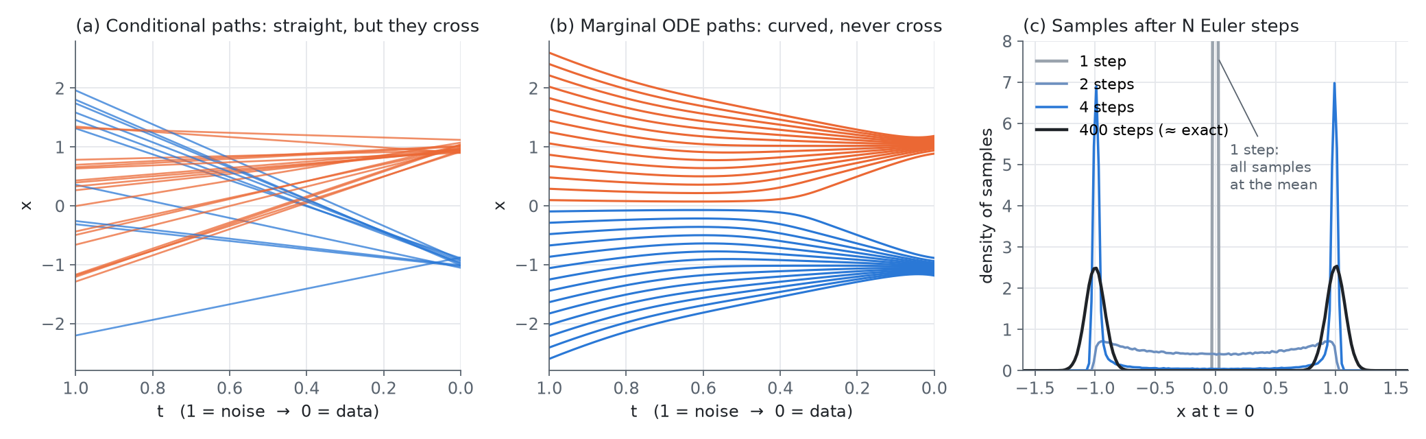
• (a) Random pairs give straight lines that cross. A noise sample at $x = 1.5$ might be paired with the mode at $-1$.
• (b) The ODE of the marginal field can’t cross (its solutions are unique), so trajectories bend: everything above 0 goes to $+1$, everything below goes to $-1$. The bend is where the posterior over modes switches.
• (c) Euler with one step gives $\hat x_0 = x_1 - v(x_1, 1) = \mathbb{E}[x_0 \mid x_1]$. At $t = 1$ the noise carries no information about the data, so that is the data mean: every sample lands at 0, between the modes. This is the blurry average you get from a one-step regression, in one dimension.

This last point is the core problem for one-step generation: the velocity at a point tells you where the average path goes, not where this sample’s path ends. Getting the endpoint needs either many small steps, a straighter field, or a network trained to predict the endpoint directly.

5. Making the field straighter

Reflow (rectified flow) #

Liu, Gong & Liu proposed: train a flow, then use it to re-pair the data. Sample $\epsilon$, solve the ODE to get $z_0 = \text{ODE}(\epsilon)$, and train a new flow on straight lines between $(z_0, \epsilon)$. These pairs come from a deterministic, non-crossing map, so the new conditional lines cross much less, and the new marginal field is straighter. They prove that each reflow does not increase any convex transport cost. After one or two reflows, few-step or even one-step Euler works much better, especially combined with distillation (InstaFlow applied this to Stable Diffusion). Lee et al. later showed that one reflow with better training (“2-rectified flow++”) is often enough.

The catch: each reflow needs a large set of ODE solves from the previous model, and errors from the teacher’s ODE compound.

Better couplings during training #

Instead of independent pairs, pair noise and data inside each minibatch by solving a small optimal-transport assignment (Tong et al.; Pooladian et al.). Paths cross less, so the field is straighter from the start. In high dimension with small batches the effect is limited, but it is cheap.

6. Practical choices that matter

Time sampling. Uniform $t$ wastes effort near $t=0$ and $t=1$, where the target is easy. SD3 samples $t$ from a logit-normal distribution, concentrated in the middle, and shifts it toward noise at higher resolution, because more pixels carry more redundant information at the same noise level:

\begin{equation} t' = \frac{s\,t}{1 + (s - 1)\,t}, \qquad s = \sqrt{m / n} \end{equation}

where $m/n$ is the ratio of pixel counts relative to the base resolution. The same shift is used for the sampling schedule.

Classifier-free guidance works on velocities like on noise predictions:

\begin{equation} \hat v = v_\theta(x_t, t, \varnothing) + w\,\big(v_\theta(x_t, t, c) - v_\theta(x_t, t, \varnothing)\big) \end{equation}

It doubles the number of network evaluations (NFE) per step unless the guidance is distilled into the model.

Solvers. Euler is the default for flow models. Heun (second order, EDM) gives the same quality with fewer steps at 2 NFE per step. With a reasonable field, 20-50 Euler steps are typical for images; video models often use 30-50 steps with CFG, i.e. 60-100 forward passes of a multi-billion-parameter transformer per sample. That cost is why the next post exists.

7. Summary

	DDPM / DDIM	Flow matching (linear path)
Path	$\sqrt{\bar\alpha_t}\,x_0 + \sqrt{1-\bar\alpha_t}\,\epsilon$	$(1-t)\,x_0 + t\,\epsilon$
Network target	$\epsilon$	$\epsilon - x_0$
Learns	$\mathbb{E}[\epsilon \mid x_t]$	$\mathbb{E}[\epsilon - x_0 \mid x_t]$
Deterministic sampler	DDIM	Euler (= DDIM on this path)
One step gives	$\mathbb{E}[x_0 \mid x_T]$ (blurry)	$\mathbb{E}[x_0 \mid x_1]$ (blurry)

Flow matching did not make diffusion faster by itself. What it did was make the object clean: a velocity field along a chosen path, trained by plain regression. The next post asks: if one step of the velocity only gives the average, can we train a network to output the endpoint of the curved path, in one step?

References

• Ho, Jain, Abbeel. Denoising Diffusion Probabilistic Models. arXiv:2006.11239
• Song, Meng, Ermon. Denoising Diffusion Implicit Models. arXiv:2010.02502
• Song et al. Score-Based Generative Modeling through Stochastic Differential Equations. arXiv:2011.13456
• Karras et al. Elucidating the Design Space of Diffusion-Based Generative Models (EDM). arXiv:2206.00364
• Lipman et al. Flow Matching for Generative Modeling. arXiv:2210.02747
• Liu, Gong, Liu. Flow Straight and Fast: Learning to Generate and Transfer Data with Rectified Flow. arXiv:2209.03003
• Albergo, Vanden-Eijnden. Building Normalizing Flows with Stochastic Interpolants. arXiv:2209.15571
• Kingma, Gao. Understanding Diffusion Objectives as the ELBO with Simple Data Augmentation. arXiv:2303.00848
• Tong et al. Improving and Generalizing Flow-Based Generative Models with Minibatch Optimal Transport. arXiv:2302.00482
• Pooladian et al. Multisample Flow Matching: Straightening Flows with Minibatch Couplings. arXiv:2304.14772
• Ma et al. SiT: Exploring Flow and Diffusion-based Generative Models with Scalable Interpolant Transformers. arXiv:2401.08740
• Esser et al. Scaling Rectified Flow Transformers for High-Resolution Image Synthesis (SD3). arXiv:2403.03206
• Lee, Lin, Fanti. Improving the Training of Rectified Flows. arXiv:2405.20320
• Lipman et al. Flow Matching Guide and Code. arXiv:2412.06264