Background

KL Divergence

KL divergence is a measure of how one probability distribution p is different from a second, reference probability distribution q. It is often denoted as $D(p||q)$

\begin{equation} D_{KL}(p||q) = \sum_{x\in X}p(x)log(\frac{p(x)}{q(x)}) \end{equation}

DDPM: Denoising Diffusion Probabilistic Models

The goal of DDPM is to construct a model to generate by denoising.

Features

1. Markov Chain

\begin{equation} p(x_t|x_{t-1},x_0) = p(x_t|x_{t-1}) \end{equation}

2. Gaussian re-parameterization \begin{align} p(x_t|x_{t-1}) \sim \mathcal{N}(x_t; \sqrt{\alpha_t}x_{t-1}, (1-\alpha_t)\mathbf{I}) \\ p(x_t|x_0) \sim \mathcal{N}(x_t; \sqrt{\bar{\alpha}_t}x_0, (1-\bar{\alpha}_t)\mathbf{I}) \\ p(x_t|x_0) = \sqrt{\bar{\alpha}_t}x_0 + \sqrt{1-\bar{\alpha}_t}\epsilon_t, \quad \epsilon_t \sim \mathcal{N}(0,\mathbf{I}) \end{align} Formula (5) is called re-parameterization, which is a key to make the model trainable.

   To be notice, in DDIM, we use $\sqrt{\alpha_t}$ instead of $\sqrt{\bar{\alpha}_t}$, which is different from the original DDPM.

3. Loss Function Goal: $\min L = -\log p_{\theta}(x_0)$

   The main loss function is:

   \begin{equation} L_{\gamma} = \sum_{t=1}^{T}\mathbb{E}_{q(x_0),\epsilon_t\sim\mathcal{N}(0,\mathbf{I})}\left[ \gamma \left\| \epsilon_t - \epsilon_{\theta}\left(\sqrt{\alpha_t}x_0 + \sqrt{1-\alpha_t},\epsilon_t’ \right) \right\|^2_2 \right] \end{equation}

Here, we directly give the formula, the derivation will be explained in appendix. Notably, the loss function is only related to $q(x_t|x_0)$

Formula

Q: What are we doing?
A: Train a network to predict $x_{t-1}$ base on $x_t$, i.e. $q(x_{t-1}|x_t)$
How? Bayesian. Since we know every time step’s $q(x_t|x_0)$ by re-parameterization, we can get following formula:

\begin{equation} q(x_{t-1}|x_t,x_0) = \frac{q(x_t|x_{t-1})q(x_{t-1}|x_0)}{q(x_t|x_0)} \end{equation}

Specifically, formula (2) is derived from the Markov Property

Q: Why DDPM is slow?
A: Markov Property. Although it offers DDPM great generative ability, it also makes the sampling process slow. Because we need to sample $x_{t-1}$ from $q(x_{t-1}|x_t,x_0)$, for every time step.

Q: How to make it fast?
A: Non-Markov Property. I will introduce DDIM(Denosing Diffusion Implicit Models) in the next section, which is a non-Markov process.

DDIM: Denoising Diffusion Implicit Models

DDIM is a non-Markov process, which can make the sampling process fast.

How to make DDPM non-Markov?

• Feature 1: We can directly apply DDIM on DDPM-trained model, which means we cannot apply a non-affine transformation to the loss function. (i.e., the $q(x_t|x_0)$ property should remain).
  • This feature means we still have the formula (5)
• Feature 2: We need to change the sampling process, i.e., the $q(x_{t-1}|x_t,x_0)$ property should be changed to avoid Markov Property.
  • Without Markov Property, the $q(x_{t-1}|x_t,x_0)$ should be redefined. Intuitively, the paper suggests the distribution to be simple (i.e., Gaussian: $\mathcal{N}(\mu(x_t,x_0);\sigma_t^2)$).
  • As a result, we use the method of indetermined coefficients to define the non-markov denoising distribution. \begin{equation} x_{t-1} = kx_0+mx_t + \sigma_t\epsilon_t, \quad \sigma_t = C, \epsilon_t \sim \mathcal{N}(0,\mathbf{I}) \end{equation}

Deduction

1. By integrating Formula (7) and (8), we can get the following equation: \begin{align} kx_0 + mx_t + \sigma_t\epsilon_t &= \sqrt{\alpha_{t-1}}x_0 + \sqrt{1-\alpha_{t-1}}\epsilon_{t-1}’ \\ kx_0 + m(\sqrt{\alpha_t}x_0 + \sqrt{1-\alpha_t}\epsilon_t’’) + \sigma_t\epsilon_t &= \sqrt{\alpha_{t-1}}x_0 + \sqrt{1-\alpha_{t-1}}\epsilon_{t-1}’ \\ \end{align}

   Notably, we cannot use simple math to solve the equation. Since $\epsilon_t$ is a random variable, we need to use the property of Gaussian distribution: $a\epsilon + b\epsilon' \sim \mathcal{N}(0,a^2+b^2)$, where $\epsilon$ and $\epsilon'$ are independent.

2. We can rewrite equation (10) as:

   \begin{equation} \mathcal{N}((k+m\sqrt{\alpha_t})x_0, (m^2(1-\alpha_t)+\sigma_t^2)\mathbf{I}) = \mathcal{N}(\sqrt{\alpha_{t-1}}x_0, (1-\alpha_{t-1})\mathbf{I}) \end{equation}

3. So, we can get the following equations:

   \begin{equation} \begin{cases} k+m\sqrt{\alpha_t} = \sqrt{\alpha_{t-1}} \\ m^2(1-\alpha_t) + \sigma_t^2 = 1-\alpha_{t-1} \end{cases} \end{equation}

4. Final formula:

   \begin{equation} q(x_{t-1}|x_t,x_0) = \mathcal{N}(\sqrt{\alpha_{t-1}}x_0 + \sqrt{1-\alpha_{t-1}-\sigma_t^2} \cdot \frac {x_t-\sqrt{\alpha_t}x_0}{\sqrt{1-\alpha_t}} , \sigma_t^2\mathbf{I}) \end{equation}

5. Since there is no Markov Property, we do not require $t-1$ and $t$ to be adjacent, i.e., we can set $t$ to be 900 and $t-1$ to be 100, which means we can skip 800 steps. This is the key to make DDIM fast.

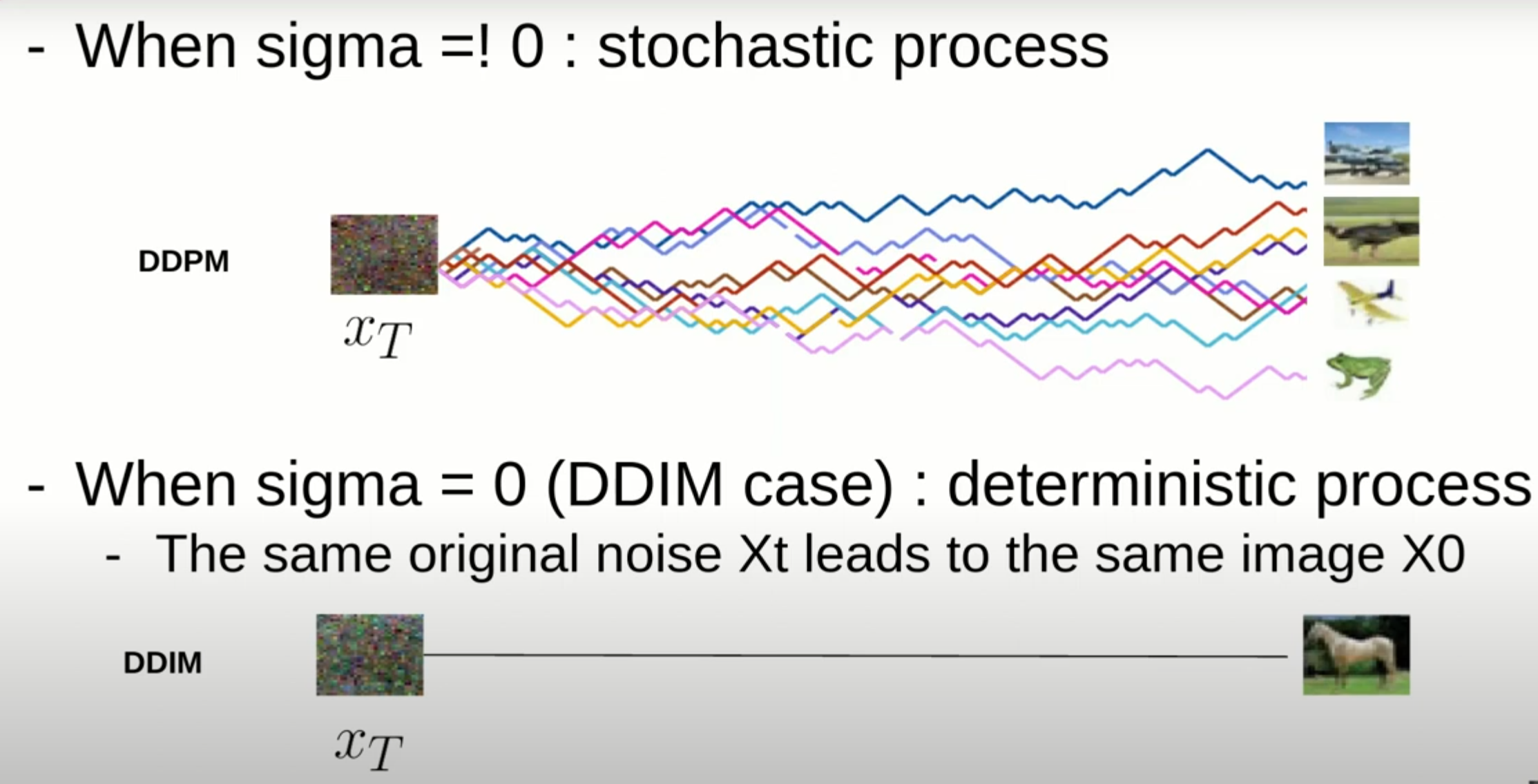
6. Finally, we have the equation (14). DDIM set $\sigma_t = 0$, i.e. no random noise. \begin{equation} x_{t-1} = \sqrt{\alpha_{t-1}}\underbrace{\left(\frac{x_t - \sqrt{1-\alpha_t}\epsilon_{\theta}(x_t)}{\sqrt{\alpha_t}}\right)}_{\text{predicted } x_0} + \underbrace{\sqrt{1-\alpha_{t-1}-\sigma_t^2} \cdot \epsilon_\theta(x_t)}_{\text{direction to } x_t} + \underbrace{\sigma_t\epsilon_t}_{\text{random noise}} \end{equation}

7. Without random noise, we can say that DDIM is not a “Diffusion” model anymore, That’s why it is called “Implicit Model”.